R for digital samling 1

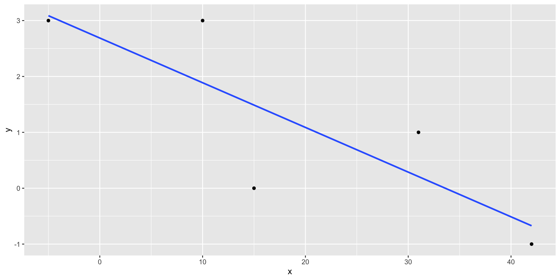
n foldnes

Pakker vi trenger å loade

library(tidyverse)
library(kableExtra)
library(broom)

Forelesningen

Lekeeksempel

x <- c(-5, 10, 15, 31, 42)
y <- c(3,3,0,1, -1)
model <- lm(y~x)
qplot(x,y)+geom_smooth(method="lm", se=F)

Lekeeksempel

summary(model)

Call:
lm(formula = y ~ x)

Residuals:
       1        2        3        4        5 
-0.08772  1.11210 -1.48796  0.79185 -0.32828 

Coefficients:
            Estimate Std. Error t value Pr(>|t|)  
(Intercept)  2.68778    0.79939   3.362   0.0437 *
x           -0.07999    0.03223  -2.481   0.0892 .
---
Signif. codes:  0 '***' 0.001 '**' 0.01 '*' 0.05 '.' 0.1 ' ' 1

Residual standard error: 1.182 on 3 degrees of freedom
Multiple R-squared:  0.6724,    Adjusted R-squared:  0.5632 
F-statistic: 6.158 on 1 and 3 DF,  p-value: 0.08916

Predikere ny verdi for \(x=20\)

yhat <- predict(model, newdata=data.frame(x=20))
yhat

       1 
1.088017 

qplot(x,y, size=3)+geom_smooth(method="lm", se=F)+geom_point(aes(x=20, y=yhat),size=5, color="red")

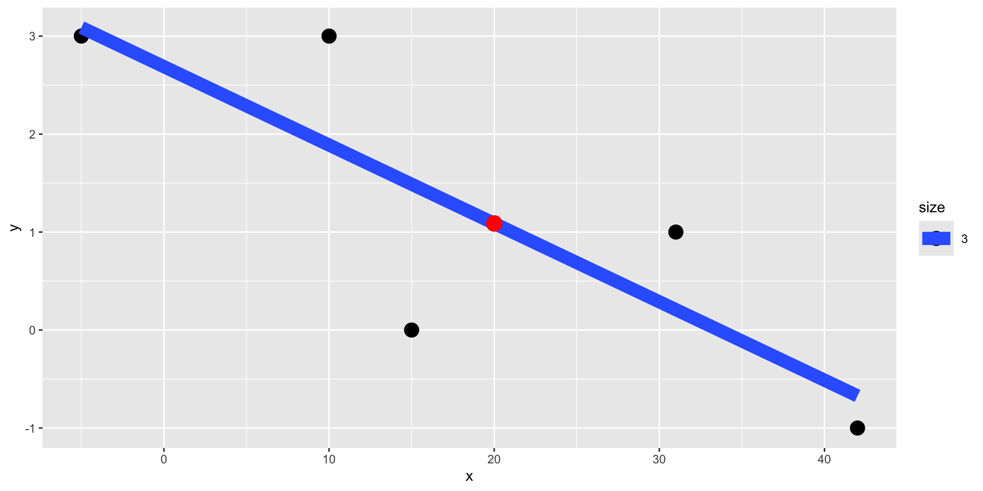
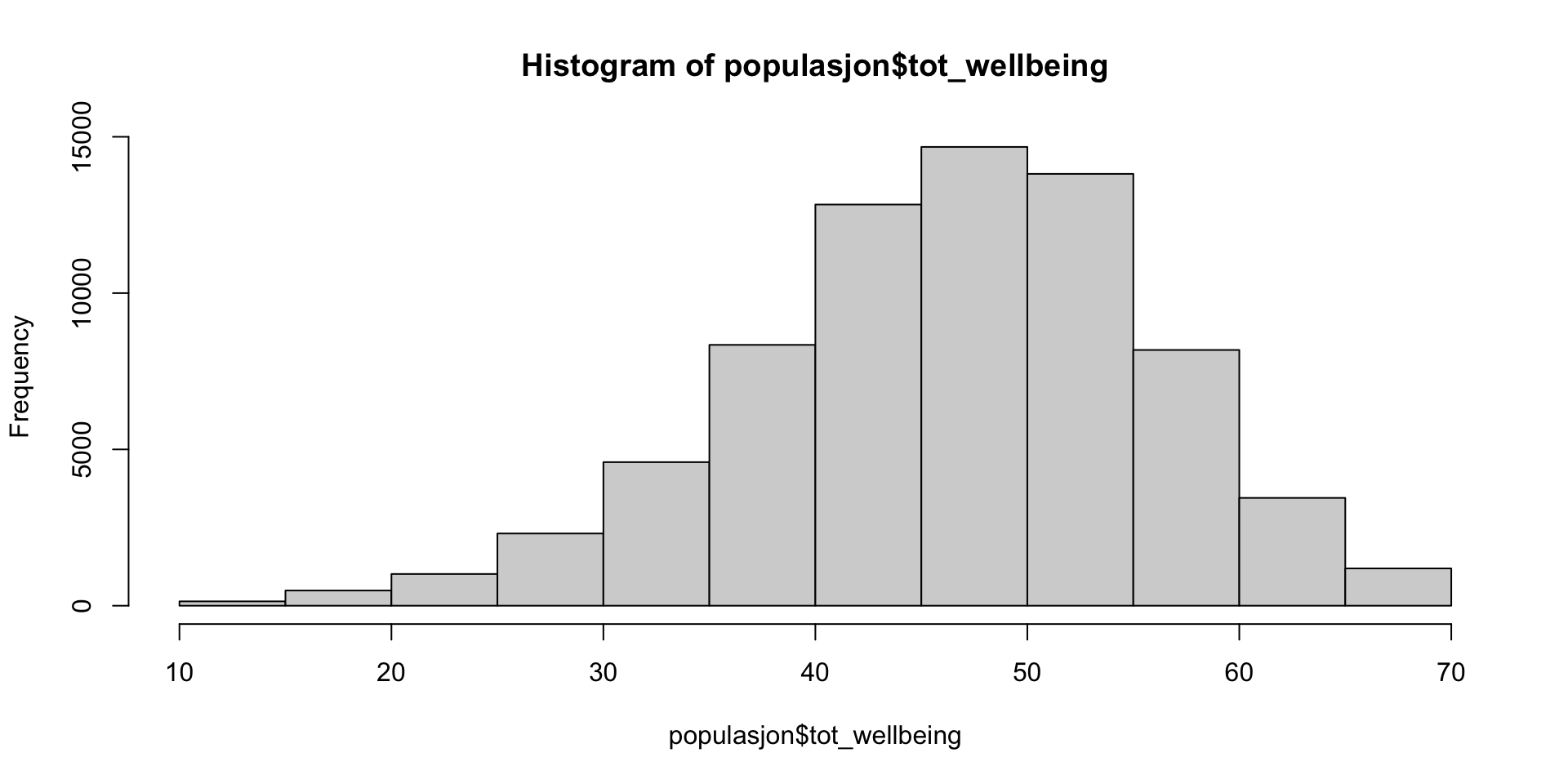
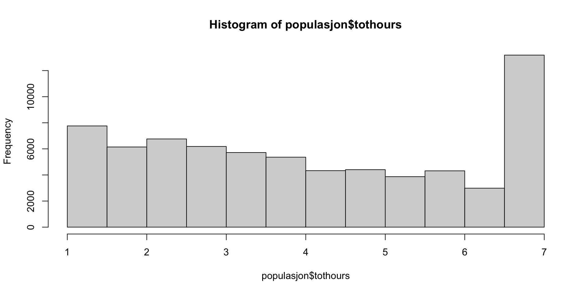
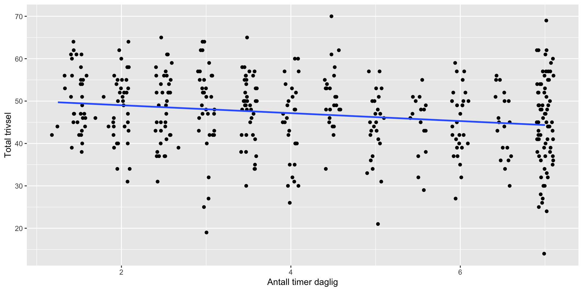
Trivsel og well-being populasjon

Last ned datasettene først! Se Data til venstre i margen

populasjon <- readRDS("../data/smartphone_wellbeing.rds")#du må endre på adressen selv. Avhenger av hvilken folder du la dataene i
hist(populasjon$tot_wellbeing)

hist(populasjon$tothours)

Regresjonen i populasjonen

popmodel <- lm(tot_wellbeing~ tothours, data=populasjon)
popmodel %>% tidy() %>% kable(digits=2)

term	estimate	std.error	statistic	p.value
(Intercept)	50.31	0.09	585.03	0
tothours	-0.81	0.02	-43.99	0

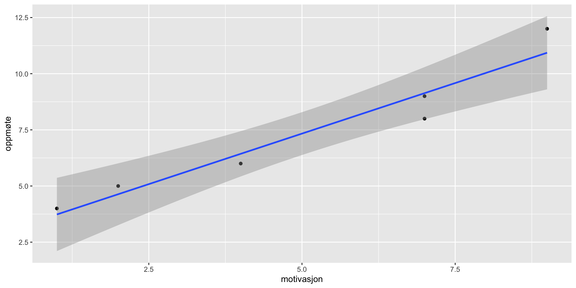
Regresjon i utvalget (last ned først)

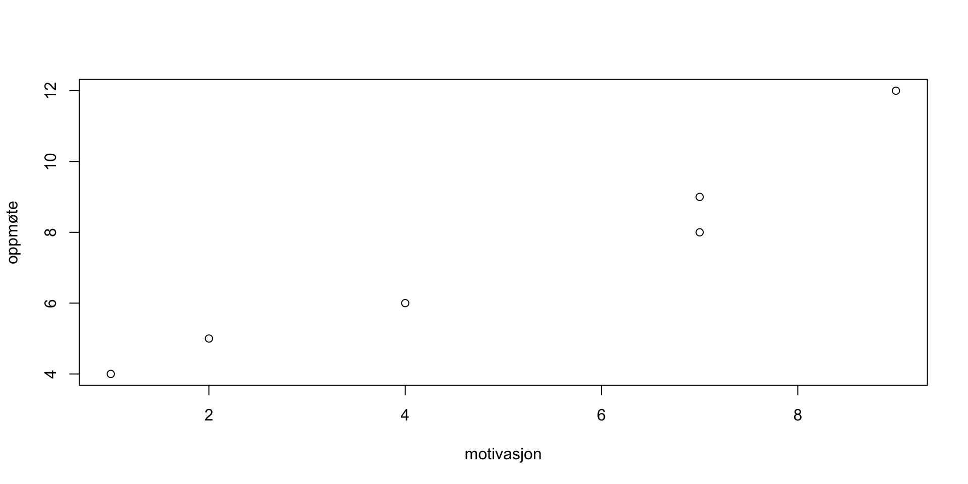
utvalg <- readRDS("../data/goldilocksutvalg.rds")
ggplot(utvalg, aes(tothours, tot_wellbeing))+geom_jitter(height=0) +geom_smooth(method="lm", se=F)+xlab("Antall timer daglig")+ylab("Total trivsel")

Regresjon i utvalget

model <- lm(tot_wellbeing~ tothours, data=utvalg)
model %>% tidy() %>% kable(digits=2)

term	estimate	std.error	statistic	p.value
(Intercept)	50.89	1.09	46.55	0
tothours	-0.93	0.23	-4.01	0

Multippel regresjon i R

\[ \text{tot_wellbeing} = \beta_0+ \beta_1 \cdot \text{tothours}+ \beta_2 \cdot \text{male}+\epsilon\]

multmodel <- lm(tot_wellbeing~ tothours+male, data=utvalg)
multmodel %>% tidy() %>% kable(digits=2)

term	estimate	std.error	statistic	p.value
(Intercept)	47.57	1.14	41.74	0
tothours	-0.69	0.22	-3.08	0
male1	6.07	0.88	6.92	0

ANOVA

aov(tot_wellbeing~ school, utvalg) %>% tidy() %>% kable(digits=2) 

term	df	sumsq	meansq	statistic	p.value
school	3	92.19	30.73	0.38	0.77
Residuals	396	32388.05	81.79	NA	NA

QUIZ

Oppg 2

motivasjon <- c(9, 4, 7, 1, 2, 7)
oppmøte <- c(12,6, 9, 4, 5, 8)
plot(motivasjon , oppmøte)

Oppg 3

sd(oppmøte)

[1] 2.94392

Oppg 4

mymodel <- lm(oppmøte~motivasjon)
mymodel

Call:
lm(formula = oppmøte ~ motivasjon)

Coefficients:
(Intercept)   motivasjon  
      2.833        0.900  

qplot(motivasjon, oppmøte)+geom_smooth(method="lm")

Oppg 6 og 7

summary(mymodel)

Call:
lm(formula = oppmøte ~ motivasjon)

Residuals:
      1       2       3       4       5       6 
 1.0667 -0.4333 -0.1333  0.2667  0.3667 -1.1333 

Coefficients:
            Estimate Std. Error t value Pr(>|t|)   
(Intercept)   2.8333     0.6872   4.123  0.01458 * 
motivasjon    0.9000     0.1190   7.562  0.00164 **
---
Signif. codes:  0 '***' 0.001 '**' 0.01 '*' 0.05 '.' 0.1 ' ' 1

Residual standard error: 0.8416 on 4 degrees of freedom
Multiple R-squared:  0.9346,    Adjusted R-squared:  0.9183 
F-statistic: 57.18 on 1 and 4 DF,  p-value: 0.001639

ID1 har residual 1.0667.

Adjusted R-squared: 0.9183: 92% av variasjon i oppmøte forklare vha av varierende motivasjon. 8% av variasjonen skyldes andre faktorer enn motivasjon

Oppg 8

MinstTo <- c(1, 0, 1, 0, 0, 1)# 1=MinstTO
mymodel <- lm(motivasjon~MinstTo)
mymodel# Vi forventer at MinstTo gir et motivasjon som er 5.33 høyere enn når MinstTO=0

Call:
lm(formula = motivasjon ~ MinstTo)

Coefficients:
(Intercept)      MinstTo  
      2.333        5.333  

Oppg 9

eksamensscore <- c(15, 7, 12.5, 3, 4.5, 11)
mymodel <- lm(eksamensscore~oppmøte)
mymodel# effekt av oppmøte: Ett ekstra oppmøte gir en forventa økning i eksamensscore på 1.577

Call:
lm(formula = eksamensscore ~ oppmøte)

Coefficients:
(Intercept)      oppmøte  
     -2.731        1.577  

Oppg 10

predict(mymodel, newdata=data.frame(oppmøte=5))

       1 
5.153846 

Oppg 12

mymodel <- lm(eksamensscore ~ oppmøte + motivasjon)
summary(mymodel)

Call:
lm(formula = eksamensscore ~ oppmøte + motivasjon)

Residuals:
        1         2         3         4         5         6 
-0.276471 -0.147059  0.747059  0.005882 -0.029412 -0.300000 

Coefficients:
            Estimate Std. Error t value Pr(>|t|)  
(Intercept)   0.1000     0.9336   0.107   0.9215  
oppmøte       0.4529     0.2965   1.528   0.2240  
motivasjon    1.0824     0.2760   3.922   0.0295 *
---
Signif. codes:  0 '***' 0.001 '**' 0.01 '*' 0.05 '.' 0.1 ' ' 1

Residual standard error: 0.499 on 3 degrees of freedom
Multiple R-squared:  0.9933,    Adjusted R-squared:  0.9889 
F-statistic: 224.1 on 2 and 3 DF,  p-value: 0.0005423

Oppg 13

Ett ekstra oppmøte gir 0.45 ekstra poeng på eksamen, gitt at vi kontrollerer for motivasjon

Oppg 14

Ett ekstra poeng i motivasjon gir en forventet økning i eksamensscore på 1.08

Oppg 15

99%