R for samling 1

n foldnes

Forelesningen

Housing dataene

Vi må installere noen pakker og da får vi Housing datafilen gjennom pakken Ecdat.

library(Ecdat)
library(tidyverse)
Housing <- Housing[, c(1:3, 10, 11:12)]# her velger vi ut søylene 1,2,3,10,11,12
#View(Housing) kikker litt på dataene

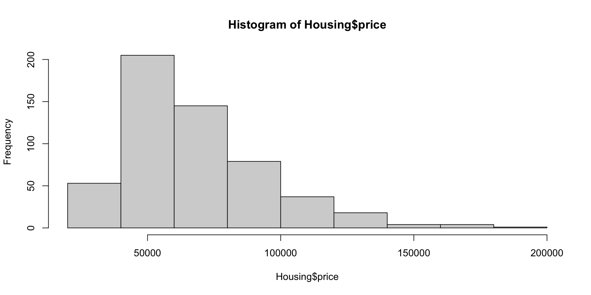
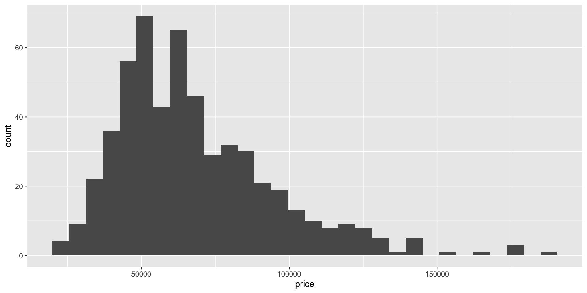
Histogram for pris

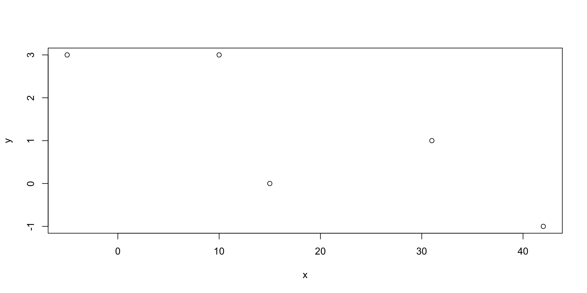
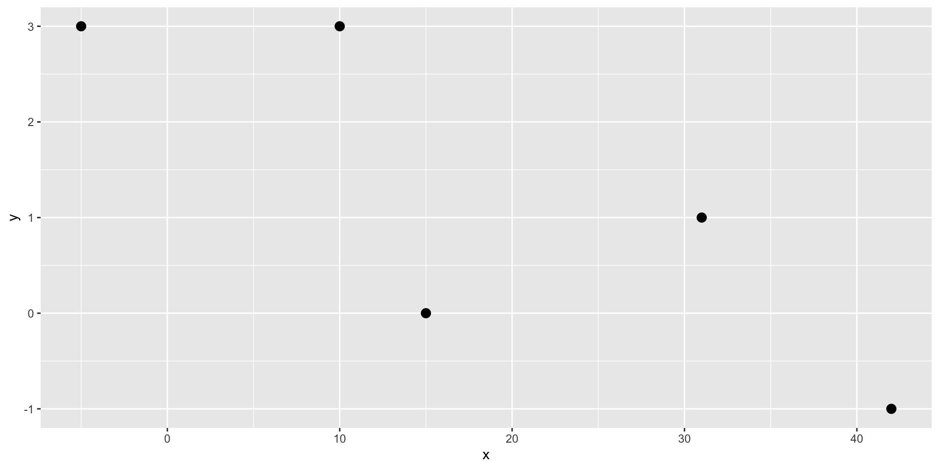
Enten bruker vi base R eller den mer kraftige pakken ggplot som vi fikk via tidyverse.

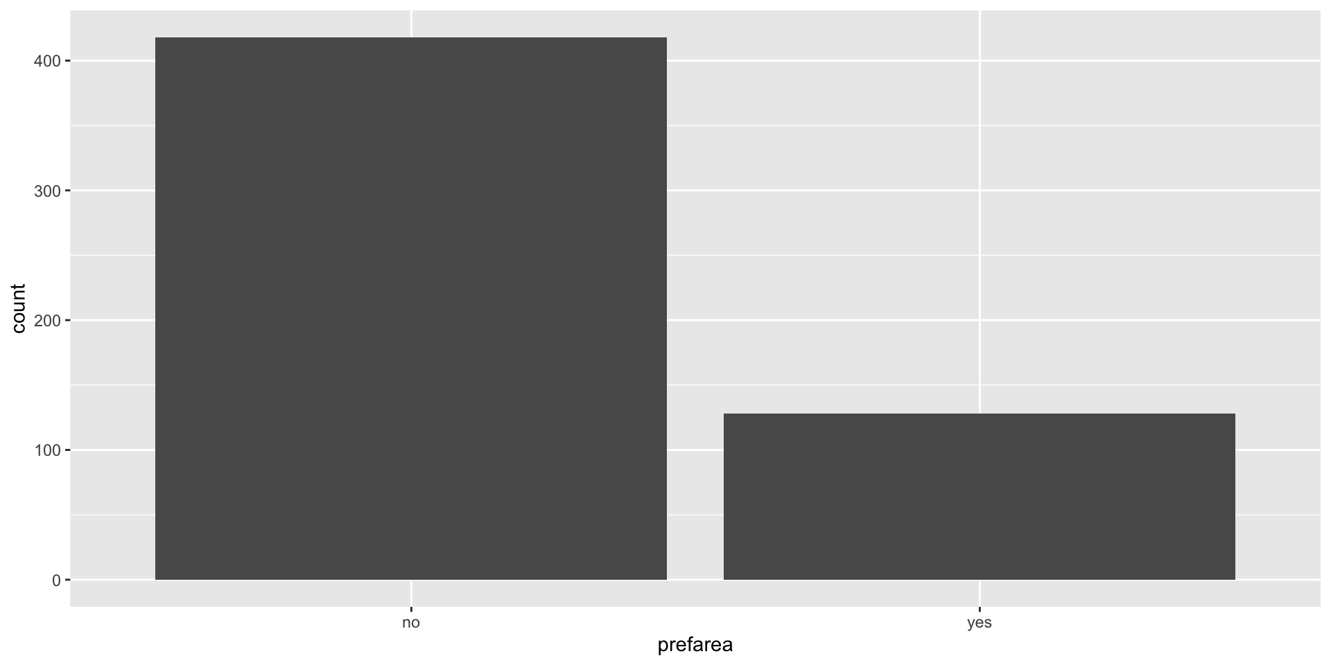
Stolpediagram for preferred area

Stolpediagram for preferred area:

#ggplot
ggplot(Housing, aes(prefarea))+geom_bar()

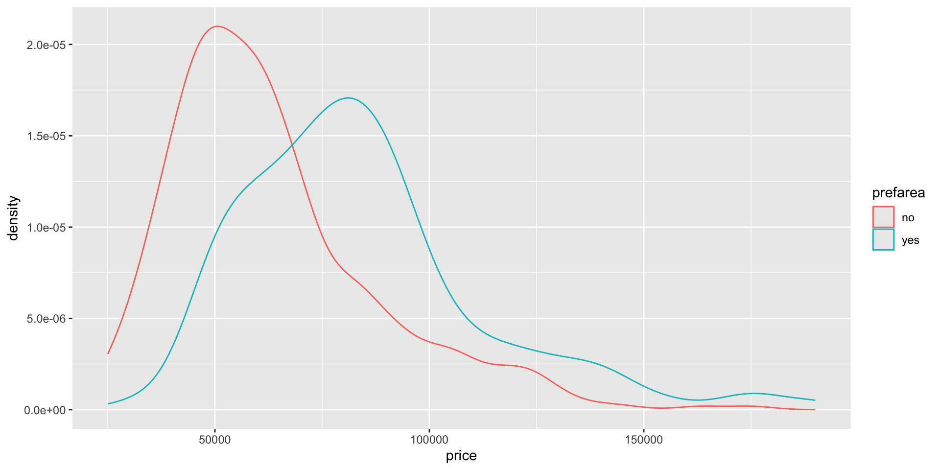
Separere på preferreed area og se på fordelingene

ggplot(Housing, aes(price, color=prefarea))+geom_density()

Alder

age <- c(16, 56, 58, 67, 62,69)

KRYSSTABELL

table(Housing$airc, Housing$prefarea)

     
       no yes
  no  298  75
  yes 120  53

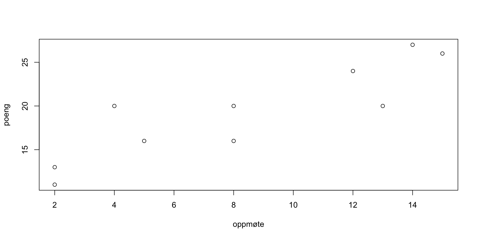
spredningsdiagram

ggplot(Housing, aes(lotsize,price))+geom_point()

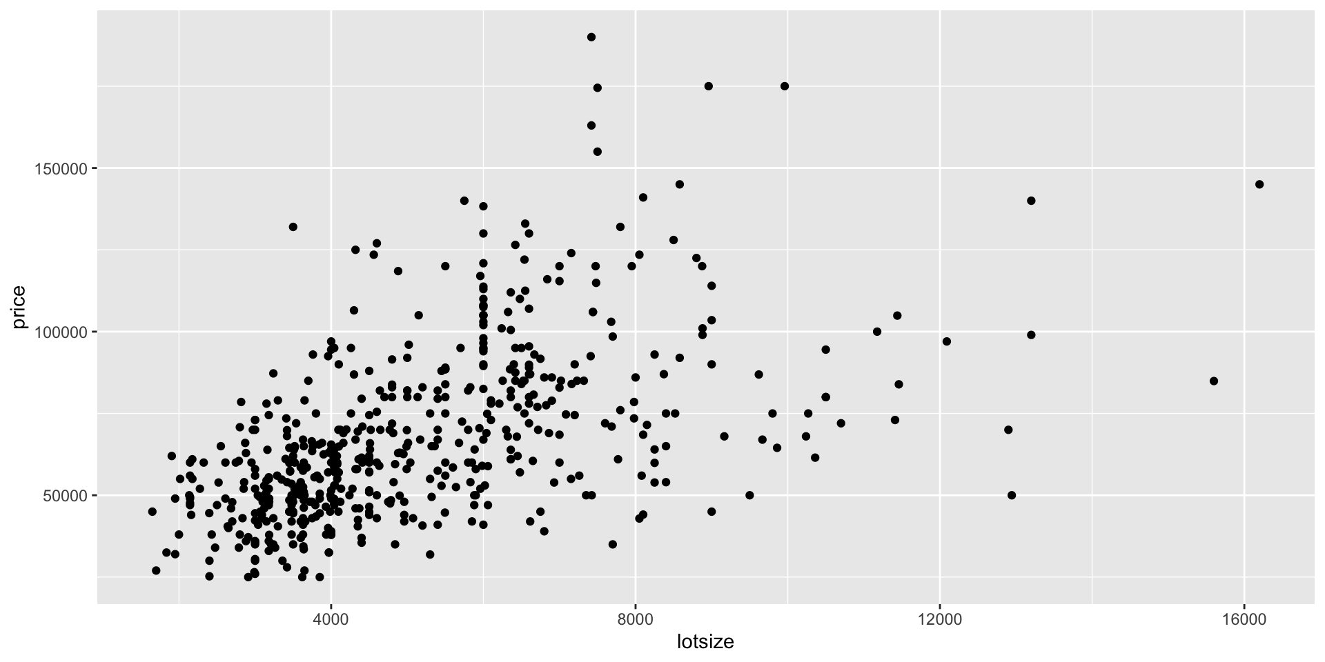
Korrelasjon

x <- c(-5 , 10 , 15 , 31 , 42)
y <- c( 3 , 3 , 0 , 1 , -1)
cor(x, y)

[1] -0.82

#base R
plot(x,y)

#ggplot
ggplot(data.frame(x,y), aes(x,y))+geom_point(size=3)

Cornflakes

vekt <- c(502, 498, 479, 492, 488, 494, 494)
t.test(vekt, mu=500)

    One Sample t-test

data:  vekt
t = -2.7105, df = 6, p-value = 0.03508
alternative hypothesis: true mean is not equal to 500
95 percent confidence interval:
 485.5935 499.2636
sample estimates:
mean of x 
 492.4286 

Quiz

Oppgave 13

alder <- c(20, 20, 19, 23, 29, 27, 25, 21)#legge inn i vektor
sd(alder)

[1] 3.664502

Oppgave 24

timer <- c(23, 55, 60, 70, 65 , 60)
sd(timer)

[1] 16.71825

Oppgave 27

prop.test(x=26, n=240)

    1-sample proportions test with continuity correction

data:  26 out of 240, null probability 0.5
X-squared = 145.7, df = 1, p-value < 2.2e-16
alternative hypothesis: true p is not equal to 0.5
95 percent confidence interval:
 0.0732806 0.1563674
sample estimates:
        p 
0.1083333 

Oppgave 28

prop.test(x=28, n=56, conf.level=.9)#stemmer!

    1-sample proportions test without continuity correction

data:  28 out of 56, null probability 0.5
X-squared = 0, df = 1, p-value = 1
alternative hypothesis: true p is not equal to 0.5
90 percent confidence interval:
 0.392661 0.607339
sample estimates:
  p 
0.5 

Oppgave 30

    One Sample t-test

data:  alder
t = 9.5681, df = 5, p-value = 0.0002112
alternative hypothesis: true mean is not equal to 0
95 percent confidence interval:
 29.61922 51.38078
sample estimates:
mean of x 
     40.5 

Oppgave 31

pinge <- read.csv("agePingelab.csv")
alder <- pinge[, 1]# bare en søyle, vi velger denne. 
mean(alder)

[1] 41.16667

Oppgave 32

t.test(alder)

    One Sample t-test

data:  alder
t = 20.769, df = 59, p-value < 2.2e-16
alternative hypothesis: true mean is not equal to 0
95 percent confidence interval:
 37.20040 45.13293
sample estimates:
mean of x 
 41.16667 

Oppgave 42

oppmøte <- c( 2 , 15 , 8 , 14, 8 , 12 , 13 , 2 , 5, 4 )
poeng <- c( 13 , 26, 20 ,27, 16, 24 , 20, 11 , 16, 20)
plot(oppmøte, poeng)

Oppgave 44

reg <- lm(oppmøte~ poeng)
summary(reg)

Call:
lm(formula = oppmøte ~ poeng)

Residuals:
    Min      1Q  Median      3Q     Max 
-4.8698 -0.8058 -0.3470  1.0486  4.1302 

Coefficients:
            Estimate Std. Error t value Pr(>|t|)    
(Intercept)  -7.4107     3.1388  -2.361 0.045887 *  
poeng         0.8140     0.1573   5.176 0.000847 ***
---
Signif. codes:  0 '***' 0.001 '**' 0.01 '*' 0.05 '.' 0.1 ' ' 1

Residual standard error: 2.527 on 8 degrees of freedom
Multiple R-squared:   0.77, Adjusted R-squared:  0.7413 
F-statistic: 26.79 on 1 and 8 DF,  p-value: 0.0008471